Examples
PHAT0
We first show the usage of GLMs to fit synthetic redshifts. We have
a dataset that has both magnitudes and redshifts for each object.
%matplotlib inline
from CosmoPhotoz.photoz import PhotoSample
Make an instance of the PhotoSample class and define the filename
of your sample
PHAT0 = PhotoSample(filename="../data/PHAT0.csv", family="Gamma", link="log")
Let’s specify the number of PCAs we want to fit and the size of the
training sample
PHAT0.num_components = 5
PHAT0.test_size = 5000
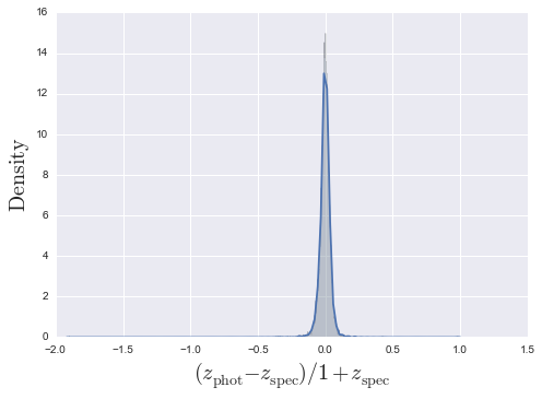
Now run the PCA decomposition and GLM fitting
PHAT0.run_full()
<matplotlib.figure.Figure at 0xb1a11a2c>
Real Data
We now show you how to use a dataset to train your GLM model and
then how to fit it to a separate testing dataset. We also show that
you can use the Quantile family rather than a Gamma family.
SDSS = PhotoSample(filename_train="../data/SDSS_train.csv", filename_test="../data/SDSS_test.csv", family="Quantile")
We note that the training set contains redshift, but the test
dataset does not contain a redshift field. We run each step
independently to show you the innards of run_all() work. Utilising
the library in an object-oriented manner allows you to interact in
a more easier manner when investigating such things as the training
sample size. See later for an example.
Applying the GLM to the SDSS
- We run principle component analysis to ensure that each
component is orthogonal (independent and identically distributed).
SDSS.do_PCA()
print("PCA has decided to use {0} components".format(SDSS.num_components))
PCA has decided to use 4 components
- First we ensure the datasets are resplit after PCA and carry out
the GLM fitting.
SDSS.split_sample(random=False)
SDSS.do_GLM()
                         QuantReg Regression Results
==============================================================================
Dep. Variable:               redshift   Pseudo R-squared:               0.8158
Model:                       QuantReg   Bandwidth:                    0.008182
Method:                 Least Squares   Sparsity:                      0.08200
Date:                Tue, 19 Aug 2014   No. Observations:                10000
Time:                        15:05:54   Df Residuals:                     9984
                                        Df Model:                           15
===================================================================================
                      coef    std err          t      P>|t|      [95.0% Conf. Int.]
-----------------------------------------------------------------------------------
Intercept           0.3156      0.000    692.656      0.000         0.315     0.317
PC1                 0.0493      0.000    385.097      0.000         0.049     0.050
PC2                -0.0322      0.001    -43.416      0.000        -0.034    -0.031
PC1:PC2             0.0045      0.000     21.331      0.000         0.004     0.005
PC3                 0.2093      0.002    103.342      0.000         0.205     0.213
PC1:PC3            -0.0213      0.000    -45.427      0.000        -0.022    -0.020
PC2:PC3             0.0409      0.001     28.324      0.000         0.038     0.044
PC1:PC2:PC3        -0.0096      0.000    -25.380      0.000        -0.010    -0.009
PC4                 0.2813      0.006     46.342      0.000         0.269     0.293
PC1:PC4            -0.0003      0.002     -0.213      0.831        -0.003     0.003
PC2:PC4            -0.2007      0.006    -31.264      0.000        -0.213    -0.188
PC1:PC2:PC4         0.0321      0.002     19.469      0.000         0.029     0.035
PC3:PC4            -0.0806      0.012     -6.999      0.000        -0.103    -0.058
PC1:PC3:PC4         0.0108      0.002      4.640      0.000         0.006     0.015
PC2:PC3:PC4        -0.0591      0.008     -7.600      0.000        -0.074    -0.044
PC1:PC2:PC3:PC4     0.0175      0.002      9.303      0.000         0.014     0.021
===================================================================================
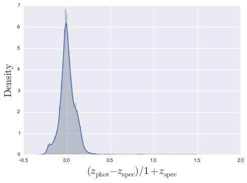
- Make a 1 dimensional KDE plot of the number of outliers.
SDSS.make_1D_KDE()
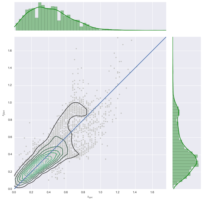
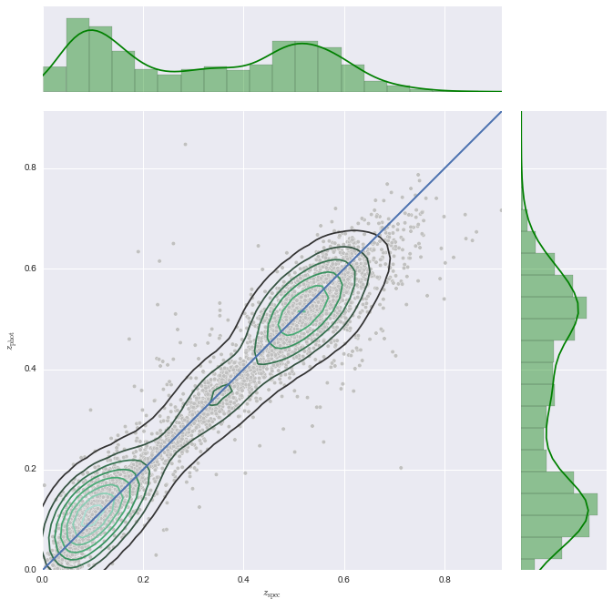
- Make a 2D KDE plot
SDSS.make_2D_KDE()
<matplotlib.figure.Figure at 0xb15ae30c>
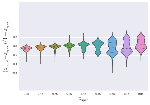
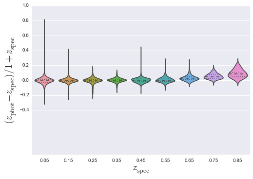
- Make a violin plot
SDSS.make_violin()
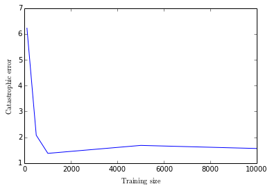
Abuse of Object-Orientation
Imagine that we want to investigate how the catastrophic error
evolves with the size of the sample used to train the Generalised
Linear Model. This can be easily carried out in an object-oriented
way, in comparison to functional forms.
import numpy as np              # for arrays
import matplotlib.pyplot as plt # for plotting

# Load a full dataset
SDSS = PhotoSample(filename="../data/SDSS_nospec.csv", family="Gamma", link="log")

# Definitions
train_size = np.array([100, 500, 1000, 5000, 10000])
catastrophic_error = []

# Run over training sizes
for i in range(len(train_size)):

    # User defined
    SDSS.test_size = train_size[i]

    # This can also be placed in a method to make cleaner
    SDSS.do_PCA()
    SDSS.split_sample(random=True)
    SDSS.do_GLM()

    # Collect the output
    catastrophic_error.append(SDSS.catastrophic_error)

# Make nicer for MPL
catastrophic_error = np.array(catastrophic_error)

# Define the figure for plotting
fig = plt.figure(0)
ax = fig.add_subplot(111)
ax.errorbar(train_size, catastrophic_error)
ax.set_xlabel(r"$\rm Training\, size$")
ax.set_ylabel(r"$\rm Catastrophic\, error$")

plt.show()
PHAT0
We first show the usage of GLMs to fit synthetic redshifts. We have a dataset that has both magnitudes and redshifts for each object.
%matplotlib inline
from CosmoPhotoz.photoz import PhotoSample
Make an instance of the PhotoSample class and define the filename of your sample
PHAT0 = PhotoSample(filename="../data/PHAT0.csv", family="Gamma", link="log")
Let’s specify the number of PCAs we want to fit and the size of the training sample
PHAT0.num_components = 5
PHAT0.test_size = 5000
Now run the PCA decomposition and GLM fitting
PHAT0.run_full()
<matplotlib.figure.Figure at 0xb1a11a2c>
Real Data
We now show you how to use a dataset to train your GLM model and then how to fit it to a separate testing dataset. We also show that you can use the Quantile family rather than a Gamma family.
SDSS = PhotoSample(filename_train="../data/SDSS_train.csv", filename_test="../data/SDSS_test.csv", family="Quantile")
We note that the training set contains redshift, but the test dataset does not contain a redshift field. We run each step independently to show you the innards of run_all() work. Utilising the library in an object-oriented manner allows you to interact in a more easier manner when investigating such things as the training sample size. See later for an example.
Applying the GLM to the SDSS
- We run principle component analysis to ensure that each component is orthogonal (independent and identically distributed).
SDSS.do_PCA()
print("PCA has decided to use {0} components".format(SDSS.num_components))
PCA has decided to use 4 components
- First we ensure the datasets are resplit after PCA and carry out the GLM fitting.
SDSS.split_sample(random=False)
SDSS.do_GLM()
QuantReg Regression Results
==============================================================================
Dep. Variable: redshift Pseudo R-squared: 0.8158
Model: QuantReg Bandwidth: 0.008182
Method: Least Squares Sparsity: 0.08200
Date: Tue, 19 Aug 2014 No. Observations: 10000
Time: 15:05:54 Df Residuals: 9984
Df Model: 15
===================================================================================
coef std err t P>|t| [95.0% Conf. Int.]
-----------------------------------------------------------------------------------
Intercept 0.3156 0.000 692.656 0.000 0.315 0.317
PC1 0.0493 0.000 385.097 0.000 0.049 0.050
PC2 -0.0322 0.001 -43.416 0.000 -0.034 -0.031
PC1:PC2 0.0045 0.000 21.331 0.000 0.004 0.005
PC3 0.2093 0.002 103.342 0.000 0.205 0.213
PC1:PC3 -0.0213 0.000 -45.427 0.000 -0.022 -0.020
PC2:PC3 0.0409 0.001 28.324 0.000 0.038 0.044
PC1:PC2:PC3 -0.0096 0.000 -25.380 0.000 -0.010 -0.009
PC4 0.2813 0.006 46.342 0.000 0.269 0.293
PC1:PC4 -0.0003 0.002 -0.213 0.831 -0.003 0.003
PC2:PC4 -0.2007 0.006 -31.264 0.000 -0.213 -0.188
PC1:PC2:PC4 0.0321 0.002 19.469 0.000 0.029 0.035
PC3:PC4 -0.0806 0.012 -6.999 0.000 -0.103 -0.058
PC1:PC3:PC4 0.0108 0.002 4.640 0.000 0.006 0.015
PC2:PC3:PC4 -0.0591 0.008 -7.600 0.000 -0.074 -0.044
PC1:PC2:PC3:PC4 0.0175 0.002 9.303 0.000 0.014 0.021
===================================================================================
- Make a 1 dimensional KDE plot of the number of outliers.
SDSS.make_1D_KDE()
- Make a 2D KDE plot
SDSS.make_2D_KDE()
<matplotlib.figure.Figure at 0xb15ae30c>
- Make a violin plot
SDSS.make_violin()
Abuse of Object-Orientation
Imagine that we want to investigate how the catastrophic error evolves with the size of the sample used to train the Generalised Linear Model. This can be easily carried out in an object-oriented way, in comparison to functional forms.
import numpy as np # for arrays
import matplotlib.pyplot as plt # for plotting
# Load a full dataset
SDSS = PhotoSample(filename="../data/SDSS_nospec.csv", family="Gamma", link="log")
# Definitions
train_size = np.array([100, 500, 1000, 5000, 10000])
catastrophic_error = []
# Run over training sizes
for i in range(len(train_size)):
# User defined
SDSS.test_size = train_size[i]
# This can also be placed in a method to make cleaner
SDSS.do_PCA()
SDSS.split_sample(random=True)
SDSS.do_GLM()
# Collect the output
catastrophic_error.append(SDSS.catastrophic_error)
# Make nicer for MPL
catastrophic_error = np.array(catastrophic_error)
# Define the figure for plotting
fig = plt.figure(0)
ax = fig.add_subplot(111)
ax.errorbar(train_size, catastrophic_error)
ax.set_xlabel(r"$\rm Training\, size$")
ax.set_ylabel(r"$\rm Catastrophic\, error$")
plt.show()